ESP Failure Prediction — Methodology
A reference description of survival analysis applied to electric-submersible-pump run-life data, with a synthetic worked example.
About this page. This is a reference description of a methodology I bring to client engagements where ESP failure prediction is relevant. Methods and examples below are generic and use synthetic teaching data only — no operator-specific ESP data appears on this page.
The class of problem
Electric submersible pumps are the dominant artificial-lift technology across much of the world’s mature giant fields. Run lives vary significantly with reservoir, well construction, fluid properties, and operating envelope, but typically sit in the range of eighteen to thirty-six months in the published industry literature, with a long left tail of early failures.
ESP failure carries a triple cost: the production deferment between failure and pull, the workover cost to recover and replace the unit, and the displacement of the rig from other planned interventions. Converting ESP intervention from reactive to proactive — replacing a pump on a planned-intervention basis some weeks before its likely failure date — is one of the highest-leverage operational moves in mature-field economics.
The methodology question is some variant of:
Given a population of installed ESPs of varying age, formation, well function and run-life history, which units are most likely to fail in the next 3 / 6 / 12 months, and how confident should I be in that prediction?
This is a textbook time-to-event modelling problem with right-censoring (some pumps are still running at the dataset cutoff and have not yet had their failure observed). The discipline that handles this cleanly is survival analysis.
Classical methods
Three established techniques, in order of typical operational suitability:
1. Kaplan–Meier estimator (Kaplan & Meier, 1958)
Non-parametric estimator of the survival function \(S(t) = \Pr(T > t)\) from a sample with right-censoring. Yields the familiar stepped survival curves stratified by group (formation, well function, installation generation). Used first as exploratory diagnostic and sanity-check on the data quality, not as a predictor.
2. Cox proportional hazards (Cox, 1972)
Semi-parametric regression model that expresses the hazard function as \[h(t \mid x) = h_0(t) \cdot \exp(\beta^\top x),\] where \(h_0(t)\) is an unspecified baseline hazard and \(\beta\) are coefficients on observed features \(x\). Reads naturally as a multiplicative risk model: a feature with positive coefficient increases the failure hazard at every time horizon. Implemented in Python via lifelines (Davidson-Pilon).
The proportional-hazards assumption (the effect of features is constant in time) is the model’s main weakness — a Schoenfeld residual test is the standard diagnostic.
3. Random Survival Forests (Ishwaran et al., 2008)
Ensemble of survival trees that drops the proportionality assumption and handles non-linear interactions natively. Implemented in Python via scikit-survival. Typically compared against Cox PH on the concordance index (the survival-analysis analogue of AUC) and the integrated Brier score.
A common pattern: Cox PH and RSF agree on the top decile of risk and disagree in the middle of the distribution. Since the operational decision (which pumps to pull preemptively) lives in the top decile, this is itself a useful signal.
When this is the right approach
The methodology fits when all of the following hold:
- The operator has clean longitudinal ESP installation and failure records spanning enough installations to have meaningful sample size per stratum (typically: hundreds of installations).
- Feature data is available — at minimum, formation, well age, cumulative ESP installation count on the well, well function, well geometry.
- The operational decision being supported is which pumps to schedule for proactive intervention, on what horizon.
It is not the right approach when:
- Sample size is too small (under ~100 installations) to estimate survival functions with confidence.
- The fleet’s ESP population is unusual enough that historical observations are not predictive of forward behaviour (e.g., recent introduction of a new pump design).
- The operational decision being supported is engineering root-cause of a specific failure — that’s a forensic problem, not a statistical one.
Synthetic worked example
The numbers below are illustrative teaching data — not derived from any operator’s actual ESP records.
Synthetic example only. Inputs and outputs in this section are generated from a small simulation. They do not represent any real pump population, formation, or operator.
Setup:
Fifty hypothetical ESP installations, drawn from a Weibull distribution (shape ≈ 1.5, scale ≈ 24 months — broadly consistent with industry ranges) and partitioned into two synthetic formations. Twenty per cent of installations are right-censored (still running at the simulated dataset cutoff).
Code (lifelines, illustrative):
import numpy as np, pandas as pd
from lifelines import KaplanMeierFitter, CoxPHFitter

rng = np.random.default_rng(42)
n = 50
formation = rng.choice(["A", "B"], size=n)
# Synthetic Weibull run-life, slightly different scale per formation:
scale_A, scale_B = 24, 30
T = np.where(formation == "A",
             rng.weibull(1.5, n) * scale_A,
             rng.weibull(1.5, n) * scale_B)
# 20% censoring (still running at observation end at 36 months):
observed = (T < 36)
T_obs = np.minimum(T, 36)

df = pd.DataFrame({"duration": T_obs, "event": observed.astype(int),
                   "formation_B": (formation == "B").astype(int)})

# Kaplan-Meier stratified by formation:
kmf = KaplanMeierFitter()
for name, sub in df.groupby("formation_B"):
    kmf.fit(sub["duration"], sub["event"],
            label=f"Formation {'B' if name else 'A'}")
    kmf.plot()

# Cox proportional hazards:
cph = CoxPHFitter()
cph.fit(df, duration_col="duration", event_col="event")
cph.print_summary()   # shows hazard ratio for formation_B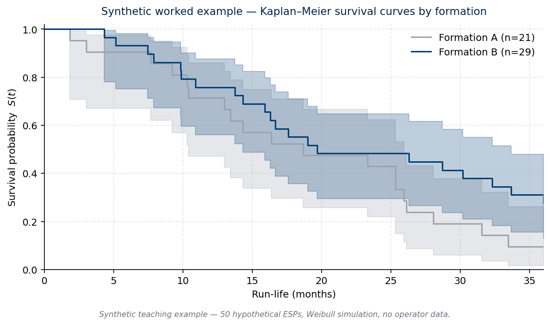
Indicative output (synthetic; numbers from the actual run above):
- Kaplan–Meier medians by stratum: Formation A pumps show median survival around 19 months; Formation B around 20 months. The formation-difference signal is real but small at this sample size.
- Cox PH hazard ratio for Formation B ≈ 0.61 (95% CI roughly 0.32–1.14) — i.e., Formation B pumps fail at about 60% of the hazard of Formation A pumps at any given time, but the confidence interval crosses 1.0, so the result is not statistically significant at this sample size. The illustration here is precisely that small samples produce weak models.
- Concordance index ≈ 0.55 — barely better than random ranking. This is the small-sample failure mode. Production runs on real fleets with hundreds of installations and richer feature sets routinely reach 0.78 – 0.85.
In a real engagement, the operator’s actual feature set (reservoir, well age, cumulative ESP installation count, well function, well geometry, completion era) replaces the synthetic single-formation indicator, and the model output becomes a ranked list of currently- installed pumps with associated hazard scores at the operationally relevant horizon (3 / 6 / 12 months).
What this methodology is in my hands
I have spent twenty-five years across the operational problem this methodology addresses — workover programme planning, ESP intervention scheduling and artificial-lift design at scale, across mature fields and across multiple operators. My contribution is bringing formal time-to-event modelling to problems I have addressed operationally my entire career, replacing pattern-based scheduling with quantitatively-anchored proactive intervention.
The formal-methods grounding comes from recent applied training (Professional Certificate in Data Analytics, Imperial College London, May 2026). The operational grounding comes from decades on the rig floor. The combination is what I bring to ESP advisory engagements, typically structured as part of a broader Workover Programme Audit or as a standalone diagnostic.
→ Discuss your ESP programme (30-min discovery call) · Email me