Workover Fleet Optimisation — Methodology

A reference description of the integer-programming approach to workover fleet capacity allocation, with a synthetic worked example.

About this page. This is a reference description of a methodology I bring to client engagements through the Workover Programme Audit service. Methods and examples below are generic and use synthetic teaching data only — no operator-specific data appears on this page.

The class of problem

A workover-fleet operator with a finite number of rigs faces an annual demand for interventions split across operational categories of varying duration and value. Each rig has finite capacity (rig-days per year), each intervention category has a different mean duration and a different non-productive-time (NPT) profile, and operational constraints set floors under certain categories (well integrity, ESP-replacement cadence) that cannot be allowed to drop.

The recurring management question is some variant of:

Given my current fleet and current NPT levels, what is the maximum annual throughput I can sustain, what mix should it deliver, and how much additional throughput would a structural change to the fleet deliver?

This is a textbook capacitated allocation problem, well-suited to integer linear programming. The formulation has been applied to upstream wells operations in the published literature since the early 2000s, and remains an active area in the SPE/OnePetro corpus.

Classical formulation

For category \(c \in \{\text{BASIC}, \text{ENHANCED}, \text{COMPLEX}\}\) (any other category set works identically):

Decision variables. Integer counts of workovers to deliver in the next planning horizon: \[n_c \in \mathbb{Z}_{\geq 0}.\]

Objective. Maximise total annual workover count: \[\max \; \sum_c n_c.\]

Constraints.

• Fleet capacity, with NPT decomposed into a fixed productive component \(p_c\) and a compressible NPT component \(t_c\), and a global NPT-reduction factor \(r \in [0, 1]\): \[\sum_{c} n_c \cdot \left( p_c + t_c \cdot (1 - r) \right) \leq N_{\text{rigs}} \times 365.\]
• Category floors (operational realities such as ESP cadence and well-integrity workover minima): \[n_c \geq C_{\min, c}.\]
• Non-negativity and integrality (implicit in the decision-variable definition).

The decomposition of duration into a productive component \(p_c\) (which cannot be compressed) and a reducible NPT component \(t_c\) (which can) is the analytical move that lets the formulation express NPT reduction as a free variable separately from category-mix rebalancing. Both levers can then be evaluated on the same footing.

Solved via PuLP with the CBC solver in Python; typical wallclock for a problem this size is under 50 ms on a 2024 laptop. No proprietary solver is required.

When this is the right approach

The methodology fits when all of the following hold:

• The operator has a finite, identifiable fleet with reasonably stable rig-day capacity.
• Intervention demand is bucketable into a small number of categories with stable mean duration and NPT profile per category.
• Operational floors (ESP cadence, integrity, regulatory minimums) are knowable and writable as linear constraints.
• The management question is a programme-level allocation decision, not a per-well sequencing decision.

It is not the right approach when:

• Per-well dependencies (zone access, equipment availability, crew rotation) dominate the calendar — in which case a scheduling formulation (e.g., a constraint-programming or RCPSP model) is more appropriate.
• The fleet is being expanded or contracted mid-year — in which case the model needs to become time-indexed.
• The operator is exploring entirely new intervention types whose duration and NPT profile are not yet characterised.

Synthetic worked example

The numbers below are illustrative teaching data — not derived from any operator’s actual workover programme.

Synthetic example only. Inputs and outputs in this section are constructed to demonstrate the methodology. They do not represent any real fleet, well, or operator.

Setup:

Parameter	Value
Fleet size	10 rigs
Annual rig-days	3,650
BASIC mean duration	10 days (1 day NPT, 9 days productive)
ENHANCED mean duration	16 days (2 days NPT, 14 days productive)
COMPLEX mean duration	22 days (3 days NPT, 19 days productive)
Minimum ENHANCED / year	100
Minimum COMPLEX / year	15

Code (PuLP, runs in under 50 ms):

from pulp import LpProblem, LpMaximize, LpVariable, LpInteger, value

N_RIGS, MIN_E, MIN_C = 10, 100, 15
CAP = N_RIGS * 365

# Productive + NPT for each category
p_B, t_B = 9, 1     # BASIC:    10 d
p_E, t_E = 14, 2    # ENHANCED: 16 d
p_C, t_C = 19, 3    # COMPLEX:  22 d

def solve(r_pct, min_complex):
    factor = 1 - r_pct / 100
    d_B = p_B + t_B * factor
    d_E = p_E + t_E * factor
    d_C = p_C + t_C * factor
    m = LpProblem("WO_MILP", LpMaximize)
    nB = LpVariable("nB", lowBound=0, cat=LpInteger)
    nE = LpVariable("nE", lowBound=0, cat=LpInteger)
    nC = LpVariable("nC", lowBound=0, cat=LpInteger)
    m += nB + nE + nC
    m += nE >= MIN_E
    m += nC >= min_complex
    m += nB * d_B + nE * d_E + nC * d_C <= CAP
    m.solve()
    return int(value(nB)), int(value(nE)), int(value(nC))

# Solve five NPT scenarios under two fleet configurations:
for r in [0, 5, 10, 15, 25]:
    fleet = solve(r, MIN_C)              # existing fleet
    ded   = solve(r, MIN_C // 2)         # half COMPLEX offloaded

Output (synthetic):

NPT reduction	Existing fleet max total	+ dedicated rig (fleet + 8 ded)	Δ
0% (baseline)	287	296 + 8 = 304	+17
−5%	289	298 + 8 = 306	+17
−10%	291	300 + 8 = 308	+17
−15%	293	302 + 8 = 310	+17
−25%	297	307 + 8 = 315	+18

Synthetic worked example — fleet capacity under MILP optimisation.

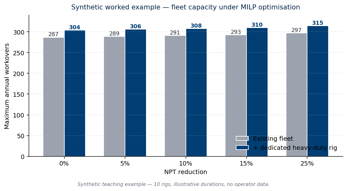
The pattern visible above is the methodologically interesting one. Under the synthetic example, NPT reduction alone adds ~10 workovers across the full reduction range (287 → 297), while offloading half the COMPLEX workovers to a dedicated rig adds ~17 workovers regardless of NPT level. This is structural: COMPLEX jobs consume the most rig-days per intervention, so removing them creates more fleet headroom than compressing NPT across all categories.

In a real engagement, the operator’s actual category mix and durations replace the synthetic numbers, the floors are set from the operator’s own operational policies, and the recommendation falls out of the solve.

What this methodology is in my hands

I have spent twenty-five years across the operational problem this methodology addresses — workover programme planning at scale, across mature fields and across multiple operators (Eni, Total, Maersk Oil, BP, Petronas Carigali, Reliance Industries). My contribution is bringing formal optimisation methods to problems I have addressed operationally my entire career, sharpening engineering judgment that would otherwise be expressed in spreadsheets and meeting-room debate.

The formal-methods grounding comes from recent applied training (Professional Certificate in Data Analytics, Imperial College London, May 2026). The operational grounding comes from decades on the rig floor. The combination is what I bring to the Workover Programme Audit service.

---

→ Discuss your workover programme (30-min discovery call) · Email me